GPCR signaling
The concept of G‑protein Coupled Receptors (GPCRs) has existed for over a century, however was not very popular among scientists at first and the fact of their very existence has been generally acknowledged by scientific community only during the latest thirty years. GPCRs represent the largest family of the membrane proteins in many species, including worms, mice, and humans. In humans there are about 800 GPCRs and they are the targets for 30%-50% of drugs prescribed worldwide. The Nobel Prize 2012 in Chemistry was awarded for studies on GPCRs to Robert J. Lefkowitz and Brian K. Kobilka [Nobel Lecture https://www.nobelprize.org/prizes/chemistry/2012/lefkowitz/lecture/].
Slide show on GPCR signaling cycle
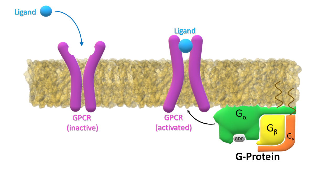
Ligand binds to the receptor (GPCR) inducing the change of its conformation to active. G‑protein binds to the activated receptor.
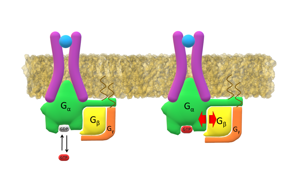
Activated G-α protein exchanges GDP for GTP. G-β and G-γ cluster separates from G-α subunit.
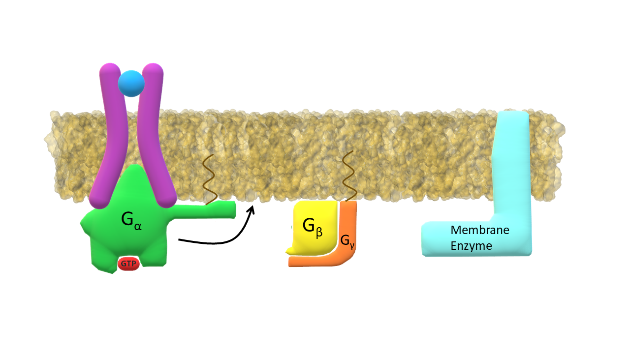
G-α subunit in active form dissociates from the receptor.
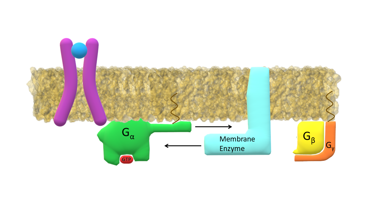
Activated G-α subunit binds to the membrane enzyme.
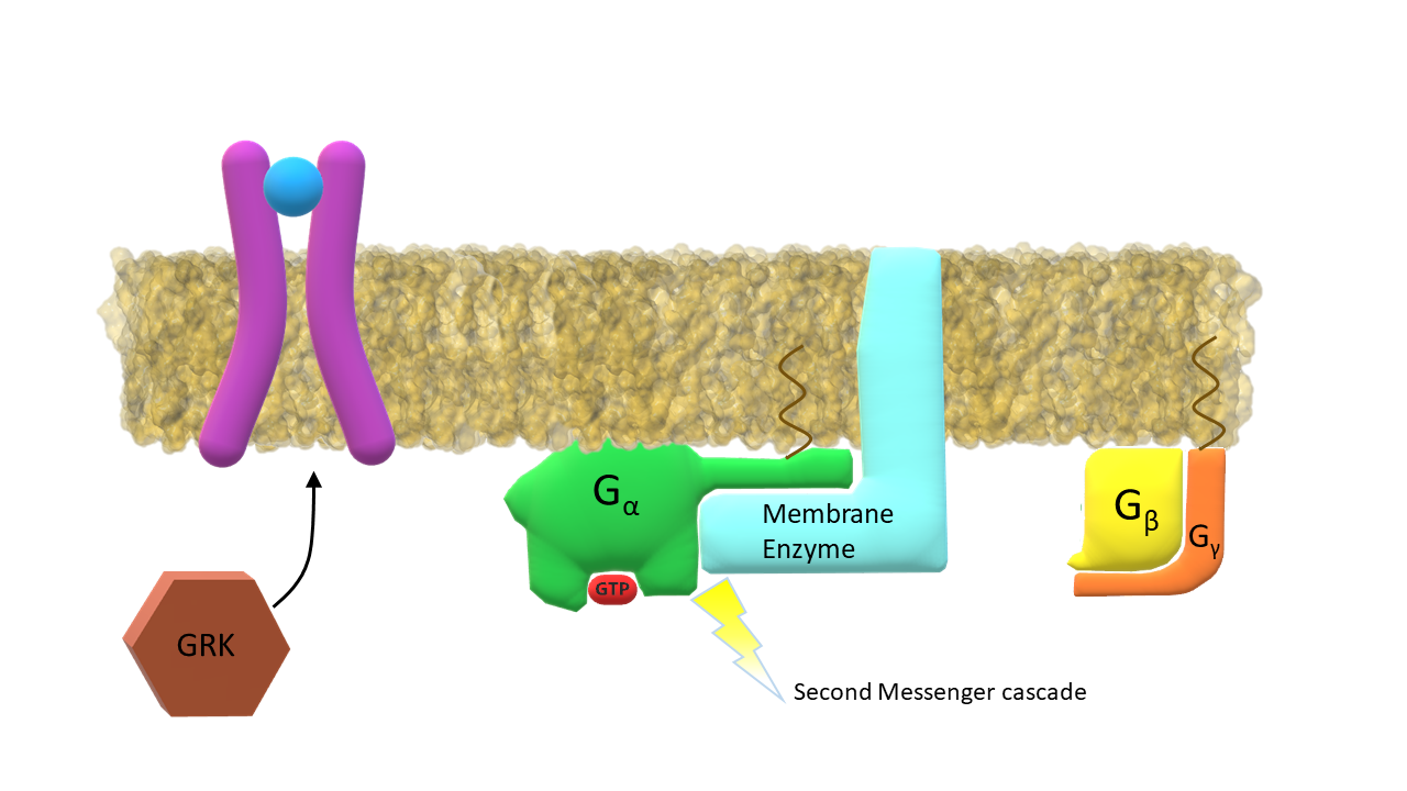
The membrane enzyme / G-α complex initiates the second messenger cascade. GPCR kinaze (GRK) binds to the intracellular side of the activated receptor.
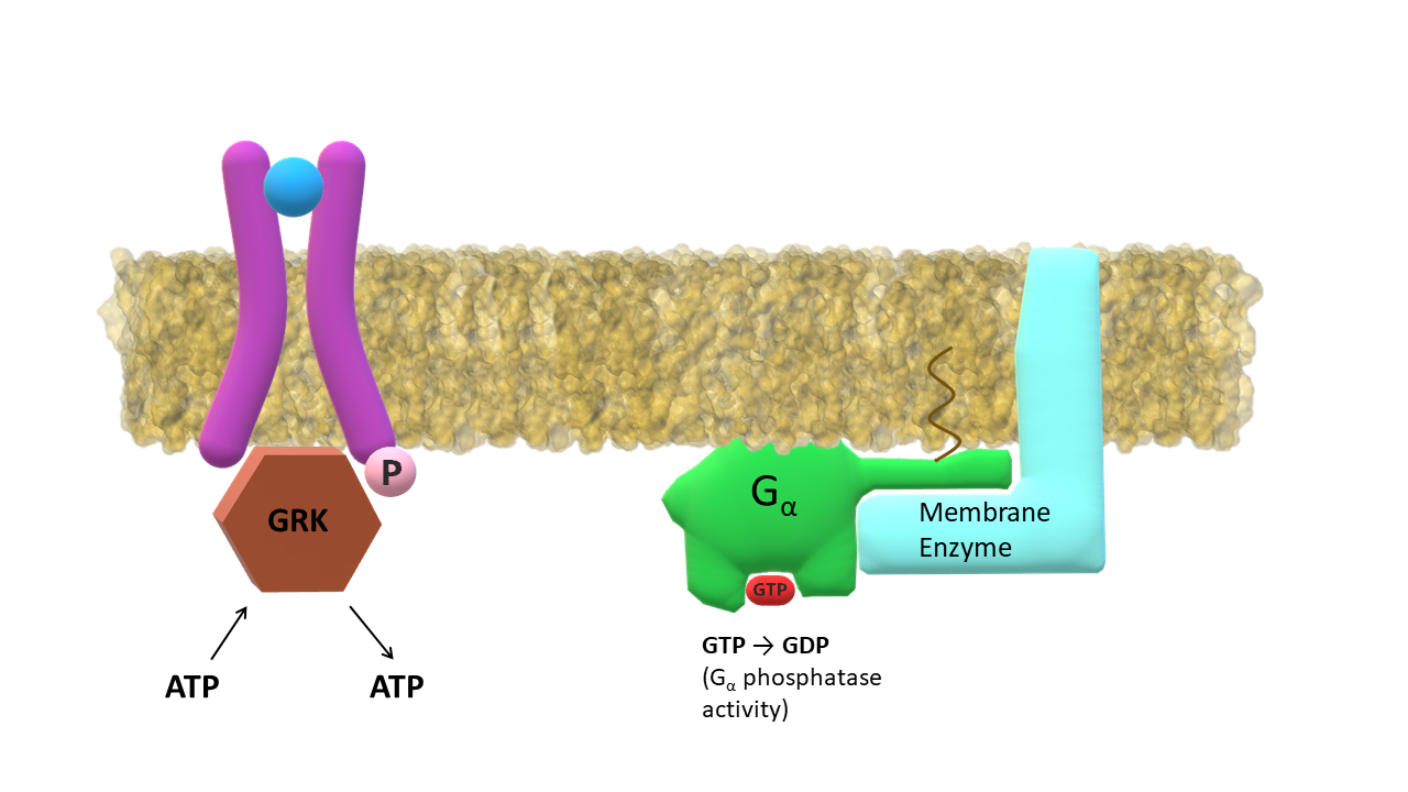
GRK phosporylates residues (Ser, Thr, Tyr) at receptor C‑terminus; G-α subunit slowly hydrolizes GTP into GDP.
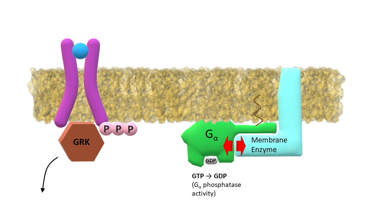
GRK dissociates from the receptor; GDP bound G‑α subunit returns to its inactive form and dissociates from the membrane enzyme.
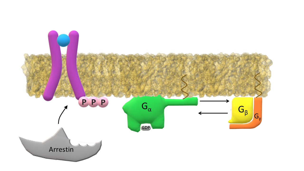
Arrestin binds to the phosphorylated intracellular end of the receptor; Inactive G‑α subunit binds again to subunits β and γ.
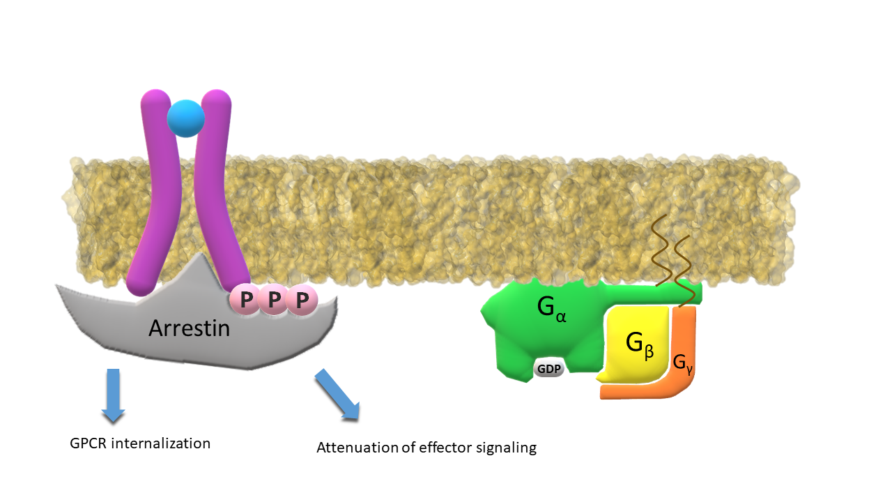
Arrestin bound to the phosphorylated receptor attenuates the effector signalling or (sometimes) initiates the receptor internalization.
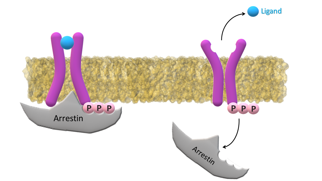
Ligand and arrestin dissociate from the receptor; Receptor returns to its inactive form.
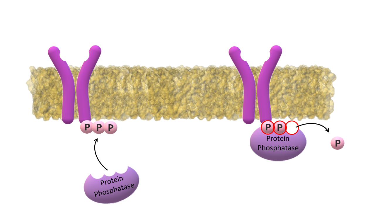
Protein Phosphatase dephosphorylates the C‑terminus of the receptor.
The GPCRsignal is a web service devoted to signaling complexes of G protein-coupled receptors (GPCRs), allowing an in silico mutagenesis and running short MD simulations of the receptor-effector protein complexes, and providing tools for analysis of the obtained trajectories. The recent improvement in cryo-Electron Microscopy resulted in determination of a large number of high resolution structures of GPCRs bound to their effector proteins: G proteins or arrestins. Currently there are 73 such complexes with determined structures but this number is quickly increasing. Analyzing the interfaces between receptor and a effector protein is of high importance since a selection of proper G protein or specific conformation of arrestin results in changes in signaling. Biased and unbiased signaling of GPCRs is of primary importance for designing more effective drugs with fewer side effects.
Tutorial
Table of contents
- Menu ‘Browse’ → <Sortable table of all available GPCR-effector protein complexes>
- Menu ‘MD&mut’ → <Molecular dynamics & mutations> page
- Menu ‘Comparison’ → <Comparison of multiple MDs> page
- Menu ‘Example 1’ → <Analysis of single MD> page
- Menu ‘Example 2’ → <Analysis of multiple MDs> page
- button ‘Details of complexes’ → <Structure information page> page
- button ‘MD preparation’ → <Molecular dynamics & mutations> page
Browsing available structures
Menu ‘Browse’ → <Sortable table of all available GPCR-effector protein(s) complexes>
When the user selects the ‘Browse’ entry (from the menu at the top) a table with all available structures of GPCR signaling complexes appears. One can select one complex and press button ‘Details of complexes’ to see more details of that complex, or to press ‘MD preparation’ to go directly to preparation page for MD simulation for that complex. Each column of the table is sortable which is very useful for making statistics of haw many complexes of particular types are currently available. To search for a certain structure(s) just type your query phrase into the ‘Search’ textbox (present in every section). You can search structures by a receptor name, effector protein name, PDB ID, organism and any other value that is included as a table column.
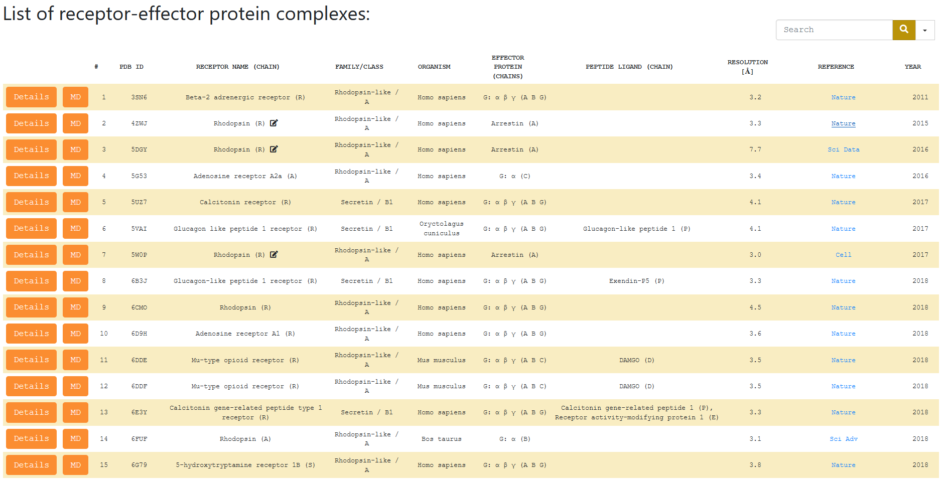
Entry number (#) – ordering number of the structures.
PDB ID (CHAIN) – a unique ID of a certain PDB structure; in parenthesis there is a letter of a protein chain of GPCR which can be different in different structures from PDB.
Receptor Name – the name of the receptor.
Family/Class – family and class of GPCR.
Organism – a Latin name of the organism from which the receptor was obtained.
Effector protein (chains) – the effector protein(s) present in the structure (with their chain letters).
Peptide Ligand (chain) – peptide ligands (with their chains) present in the complex.
Resolution – resolution of the structure (in Angstroms).
Reference – a link to the article in which the structure has been described.
Year – the year of structure deposition.
Note: Icon next to the ‘Receptors Name’ means that the structure PDB file has been
modified e.g. to distinguish chain letters of receptor and effector protein if they are originally fused and have the same chain letter.
In each case all changes are described in the 'Details of complexes' page.
‘Structure information page’ page
button ‘Details of complexes’ → <Structure information page> page
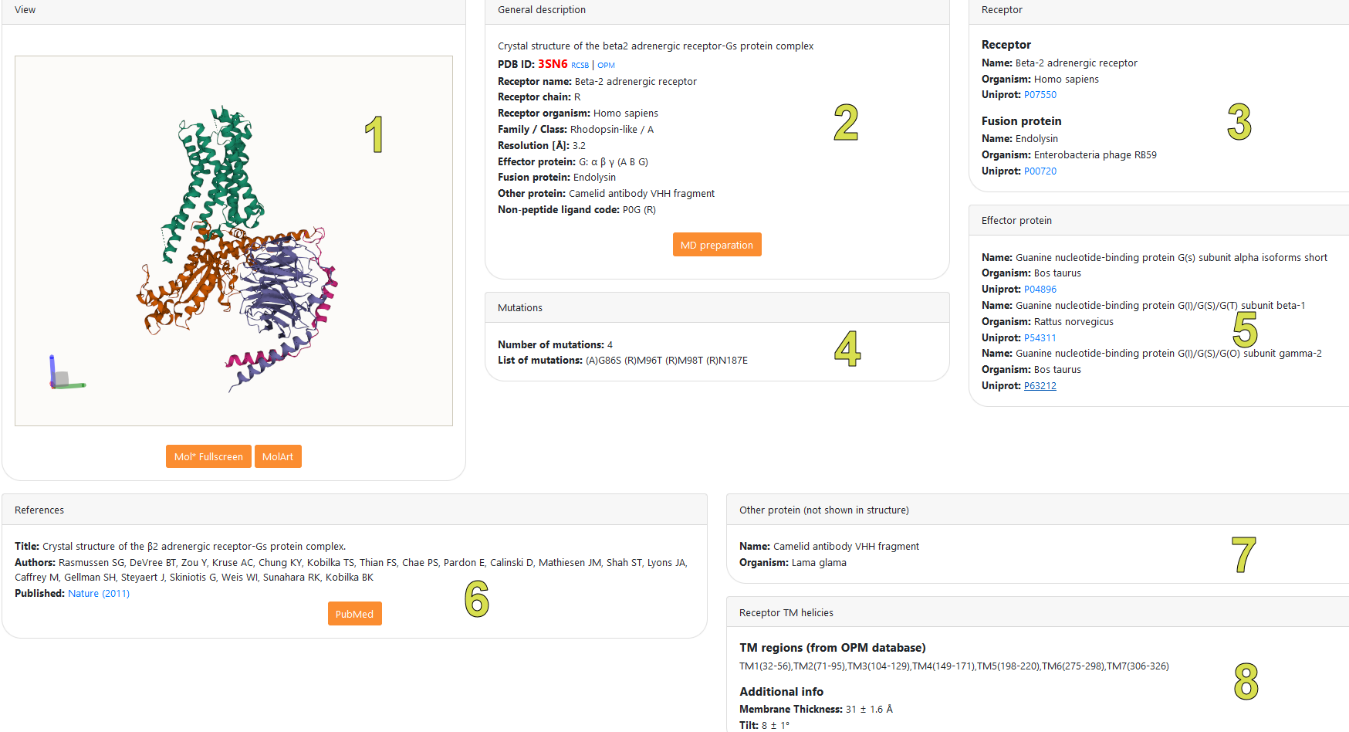
After clicking button, located on the left of the entry number ‘#’, the structure information page for that entry will be displayed:
Clicking the button brings up the full screen visualization of the chosen complex structure (in Mol*)
MolArt button brings up the visualization of the chosen receptor in MolArt: a molecular structure annotation and visualization tool (https://github.com/cusbg/MolArt). Note: MolArt identifies the structure by Uniprot ID of the receptor (and not by PDB ID of a particular complex), and will open all available structures containing that receptor (both with and without effector protein(s)). For example for the structure PDB ID: 3sn6 in GPCRsignal all structures of the human β2 adrenergic receptor will be opened in MolArt (i.e. 2r4r, 3kj6, 2r4r, 3sn6, 7dhi, etc.). Therefore the user should make sure to select the correct structure from the PDB ID menu in MolArt (shown on the screenschot below).
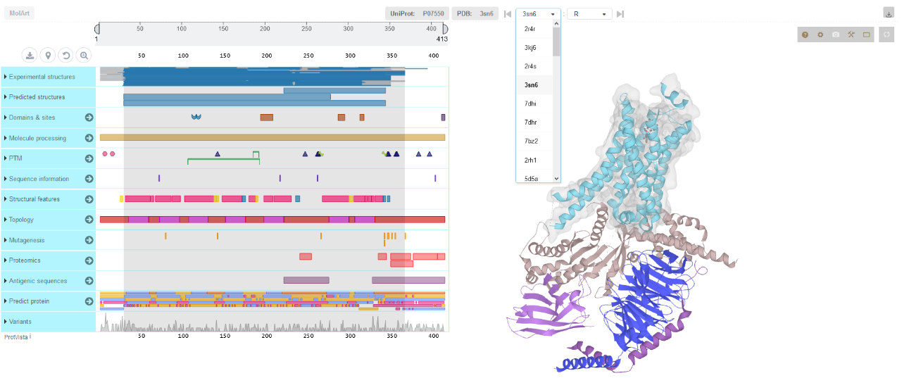
More information about MolArt viewer can be found here: https://doi.org/10.1093/bioinformatics/bty489
Clicking the button takes the user directly to the <Molecular dynamics & mutations> page where the selected complex structure is used as an input for MD simulation
Clicking the button redirects the user to the reference article in the PubMed database
View - A 3D representation of the structure in Mol* viewer
General description – basic information about the structure, such as the structure name, receptor’s name, class and family, PDB ID, effector proteins included in the complex, resolution of the structure, ligand code etc.
Receptor – information about the receptor present in the structure (if the receptor is not present in the structure this tile is not visible). This tile contains the receptor’s name, information about the organism from which the receptor was obtained and links to UniProt sequence database. This tile also contains information about a fusion protein (if present).
Mutations – information about the artificial mutations introduced into the structure.
Effector protein – information about all the effector proteins present in the structure together with UniProt links.
References – a reference to the article in which the structure was published
Other protein (not shown in the structure) – information about components other than receptor or effector protein (if any) present in the structure in PDB. Some parts, e.g. antibodies, are removed for simulation in this service.
Receptor TM helices – information about positioning of the receptor in a membrane (membrane thickness, tilt and the range of transmembrane residues for each receptor transmembrane helix).
‘Molecular dynamics & mutations’ page:
button ‘MD preparation’ → <Molecular dynamics & mutations> page
button ‘MD’ → <Molecular dynamics & mutations> page
Menu ‘MD&mut’ → <Molecular dynamics & mutations> page
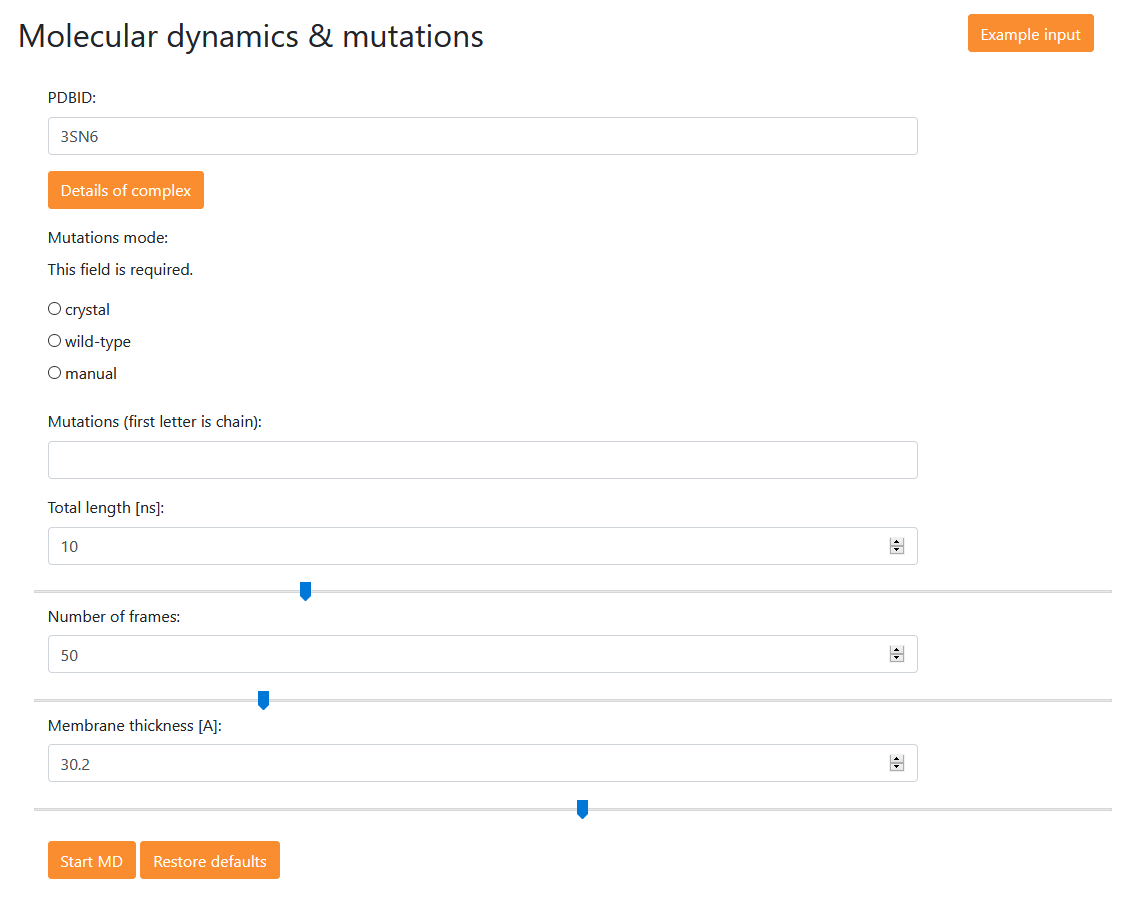
Here, the user can prepare simulation of a selected complex (being a wild type structure, a structure with crystal/cryo-EM mutations, or a structure with mutations introduced by the user). The simulations are performed in the implicit water-membrane environment (IMM1 method from CHARMM) so they are performed rather quickly.
Description of fields:
-
PDB ID: Here the user provides a PDB ID of the complex structure from the table (via Browse menu)
-
Mutation mode (crystal or cryo-EM/wild-type/manual): here the user specifies the sequence variant of a selected complex; (a) crystal or cryo-EM structure – the mutations introduced for crystallization are present in the structure, (b) wild-type – the structure is converted to a wild-type (crystallization mutations are reversed), (c) manual – user can define custom mutations in the line ‘Mutations’
-
Total length – user specifies a total length of the simulation (in nanoseconds)
-
Number of frames – user specifies how many frames are there to be in the simulation
-
Membrane thickness – user specifies the thickness (in [Å]) of the implicit membrane used in the simulation. The predicted membrane thickness for any complex can be found after clicking button Details of complexes in the list of all complexes.
(values in fields 3-5 can be adjusted using a slider below each field)
The button provides a sample data for a mutant of the cannabinoid receptor: RR145A, RR226A, AD350A, AF354A. The mutations are specified one by one in a one letter code with the first letter being the protein chain. The chains for particular proteins of the complex can be found either in the table of all available complexes via Browse menu or by selecting the complex, pressing a button , and moving the mouse pointer over the structure of the complex.
Pressing button at the bottom of the page leads to the verification page where the user is asked to provide a "Job description", email address (optionally) and to confirm the selected settings.
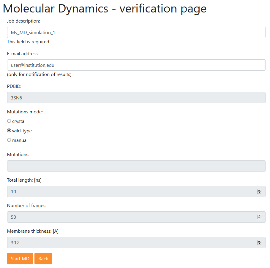
Pressing once again will start a simulation. While waiting for the results the user is redirected to the Results page <Analysis of single MD> for analyzing a single MD trajectory (identical in function to Menu: Example 1).
‘Comparison of multiple MDs’ page:
Menu ‘Comparison’ → <Comparison of multiple MDs> page

Here is the input page for selecting MD trajectories for analyses. The user is asked to copy and paste the job tokens for MD simulation(s) to be analyzed into the empty table (only simulations performed in GPCRsignal service can be analyzed or compared!). If only one job token is provided the button leads to the <Analysis of single MD> page which is illustrated by ‘Menu: Example 1’. If two or more job tokens are provided the button leads to the <Analysis of multiple MDs> page which is illustrated by ‘Menu: Example 2’.
Note: There is no particular limit for the number of MD simulations that can be included in the comparison. When a job token is pasted into bottom most field of the table, another field pops out below.
‘Analysis of single MD’ page:
Menu ‘Example 1’ → <Analysis of single MD> page
Here, the analysis of a single MD trajectory (obtained from a simulation performed in GPCRsignal) can be done. In case of Example 1 this is a simulation of a wild type CB1 cannabinoid receptor complex with G protein (PDB id: 6KPG). The residue-residue interactions between the receptor and the effector protein(s) are visualized in FlarePlot (https://gpcrviz.github.io/flareplot/). The user can select which types of interactions are to be shown (All, Salt bridges, Hydrogen bonds, Aromatic, Van der Waals). The residues are labeled using the one letter code (and capital letters while small ‘s’ and ‘t’ letters stand for the phosphorylated serine and threonine respectively). The following system is used: <chain_letter>:<residue_letter><residue_number>, so for example R:T229 means threonine 229 from chain R. The color of a residue represents the segment (protein chains) it belongs to and is identical to the color used for that segment in the structure viewer (to the right). The FlarePlot is coupled with the structure viewer so when a Play button is pressed both FlarePlot and the complex structure are updated to show (i) the changing interaction pattern in the interface between receptor and effector protein(s) in FlarePlot, and (ii) the structure of the complex in a particular frame of the trajectory in the structure viewer.
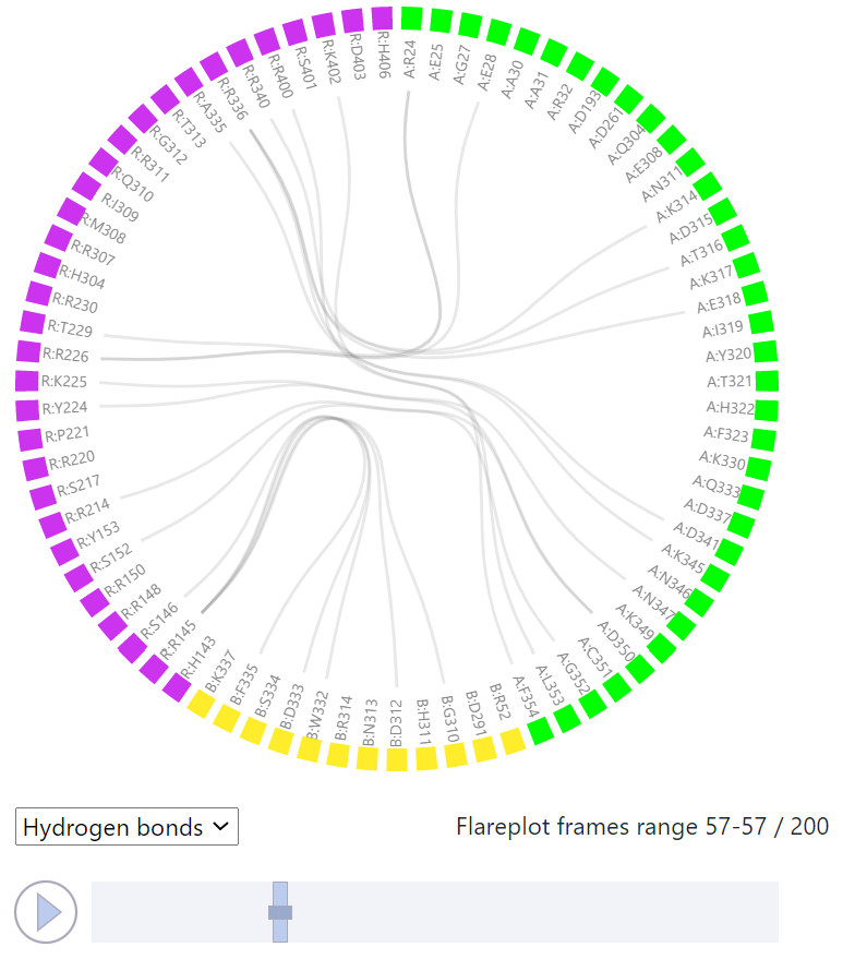
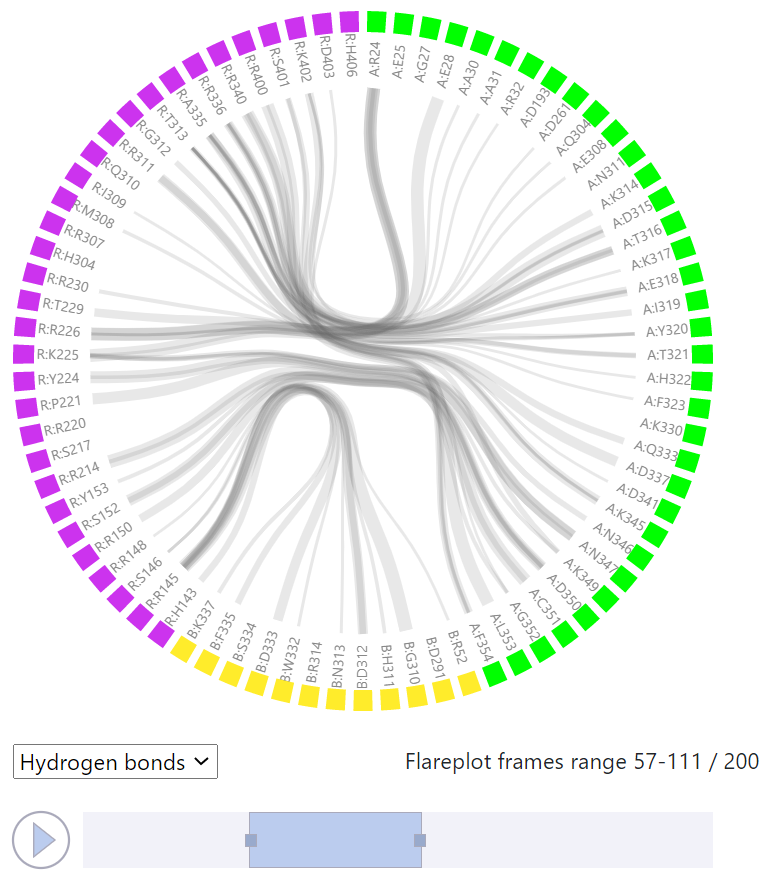
One can also select the trajectory frame to be visualized in FlarePlot by moving the the slider left or right directly with a mouse. By moving the edges of the slider left or right one can adjust the range of frames for which the interactions are shown. The line thickness corresponds to the frequency of a particular residue-residue interaction (precisely to how many times that interaction is found within the selected trajectory window). By clicking on a residue label one can highlight all the lines (interactions) that this particular residue participates in.
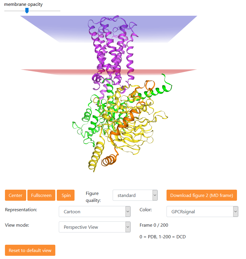
The structure of the complex is shown with red and blue semi-transparent surfaces denoting the lower and upper membrane edges. One can change the opacity of the membrane edges with a small slider above the structure viewer. The menu below the structure viewer allows for centering, showing on full screen, and spinning the structure. One can also change the figure quality (Standard, High, Very high), protein representations (Backbone, Surface, Cartoon, Licorice, Cartoon+Licorice, Spacefill, Line), color (GPCRsignal (colors as above), Rainbow, By element, By residue, By secondary structure, By hydrophobicity), and view mode (Perspective, Orthographic). Frame 0 is always a PDB structure while the rest comes from the MD simulation.
Downloads:
- Download the trajectory package as zip file containing trajectory (in DCD format) and the files for making flare plots and frequency analyses (button: above the flare plot)
- Download a current view of the flare plot (button above the flare plot)
- Download and a view of the structure (button below the structure viewer)
Clicking the button will make the results of this particular MD simulation available to other GPCRsignal users (by menu entry ‘Shared jobs’).
<Analysis of multiple MDs> page:
Menu ‘Example 2’ → <Analysis of multiple MDs> page
Here, the analysis of multiple MD simulations can be done. This page is identical in function to Example 2 where two simulations of a wild type and two simulations of mutant CB1 cannabinoid receptor complex with G protein (PDB id:6KPG) can be analyzed and compared (mutations: RR145A, RR226A, AD350A, AF354A, the first letter denotes the protein chain).
User can navigate to a single simulation view by clicking button next to each of the presented simulations. A job token and a user description for a particular simulation are specified.
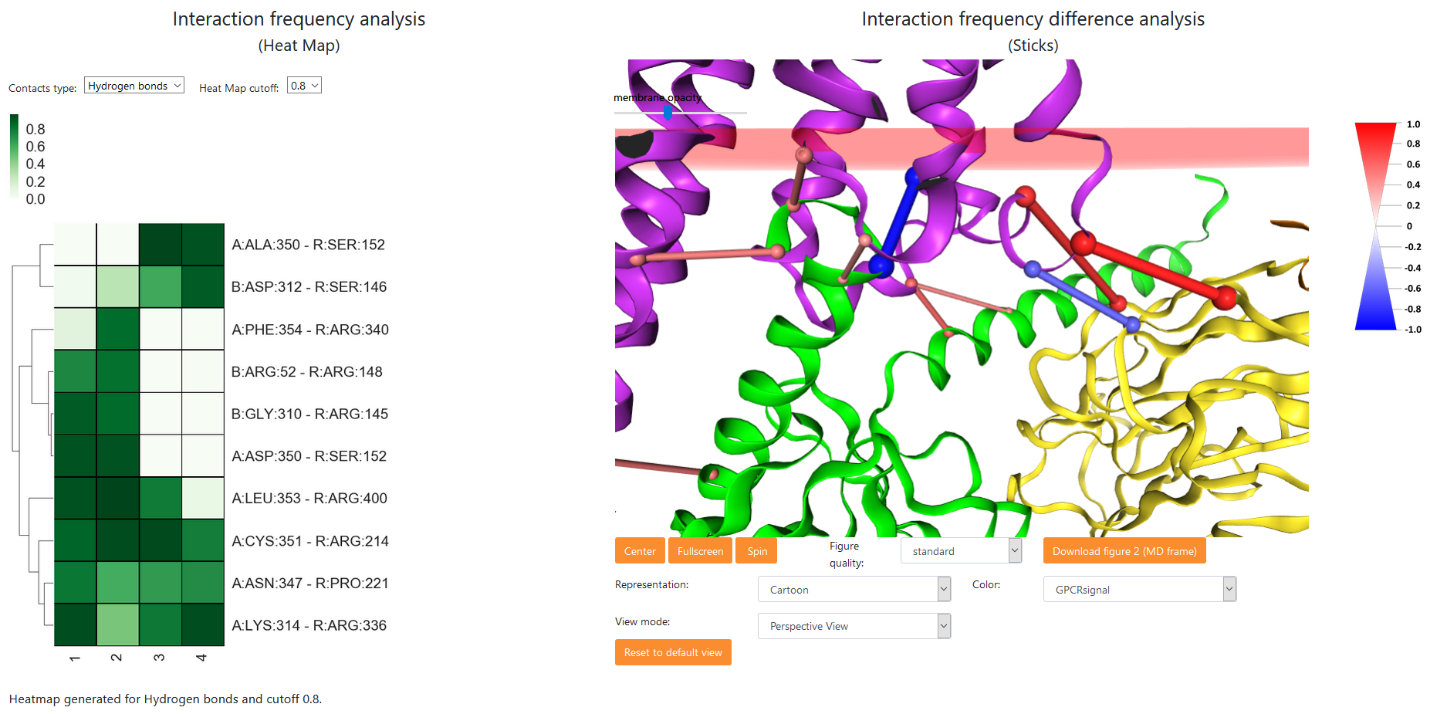
For all simulations a HeatMap is calculated for a selected type of interaction (Hydrogen bonds, salt bridges, Aromatic) and for selected cutoff. The heatmap cutoff 0.5 means that only those interactions having frequency of occurrence of 0.5 (or higher) in at least one of the analyzed MD simulations are shown. The scale bar above the heatmap shows colors used to illustrate the interaction frequencies in range 0-1, with 0 meaning no interaction in any frame of particular MD simulation, and 1 meaning that this interaction is present in all frames of that particular trajectory.
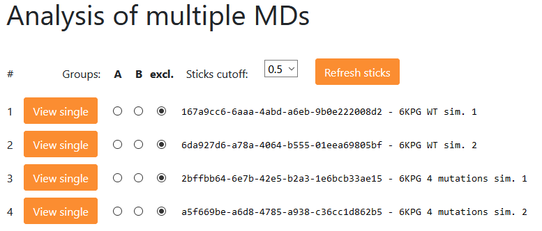
The interaction frequency difference can be calculated for two sets of MD simulations. After selecting the trajectories into groups A and B (by default all groups are empty) the user should click the button. The difference of average frequencies between groups is then calculated for each interaction (if each group contains only one trajectory, the frequency differences between those two trajectories are calculated) and visualized in a form of red and blue sticks linking the Cα atoms of interacting residues. Only the meaningful interactions are shown based on the frequency difference cutoff which can be set by the user (default sticks cutoff is 0.5). After changing the cutoff the user should click the button once again in order to redraw sticks using the new cutoff value. The intensity of a color and the thickness of a stick are proportional to the average frequency difference between groups A and B for that particular interaction. Color/thicknes scale is shown on the right side of the image.
The user can download the results for each task as a ZIP archive including basic files: protein structure (PDB/PSF format), result of molecular dynamics (DCD format), job information file (a text file containing various information about the simulation, such as job parameters etc.), contacts files (format: tab-separated values), Flareplot files (json format). Protein files are ready to use with corresponding DCD file if the user wants to visualize the trajectory in an external visualization software. Protein result files depend on selected wild-type or crystal / cryo-EM structure mode and includes user introduced mutations. A job token found in the job information file can be used to visualize the results of a particular simulation on GPCRsignal server and make analyses (valid for two months since computation).
We supply files describing all contacts between a receptor and effector proteins during simulation (tab-separated contact frequency files and Flareplot json files). Flareplots can be generated any time (even after the two months period) by uploading those json files on the page: https://gpcrviz.github.io/flareplot/?p=create.
Menu ‘Shared jobs’ → <Shared jobs list> page
Clicking the ‘Shared jobs’ leads to a GPCRsignal trajectories data base. The trajectories from MD simulations performed by the users who agreed for their results to be available for public are kept here. In order to submit your results to the ‘Shared jobs list’ on the ‘Analysis of single MD’ page click button.